Biological learning toy
The Fly's Trick
A small MNIST experiment inspired by the fly olfactory system: expand into many sparse random features, keep a tiny active tag, and learn with a simple local readout.
The fly olfactory circuit has a surprisingly useful computational pattern: project a compact sensory input into a much larger population, keep only a small sparse set of active cells, and let downstream neurons read out that sparse tag.
Plainly: the fly turns a small smell signal into a big sparse code that is easier to learn from.
I wanted a tiny artificial version of that idea. Not a biologically faithful fly model, and not an MNIST benchmark. Just a clean mechanism test: if I turn each digit into a sparse "Kenyon-cell-like" tag, how much structure does that tag preserve before any deep training?
Plainly: this is a mechanism demo, not a claim that the toy is a real fly model or a strong MNIST system.
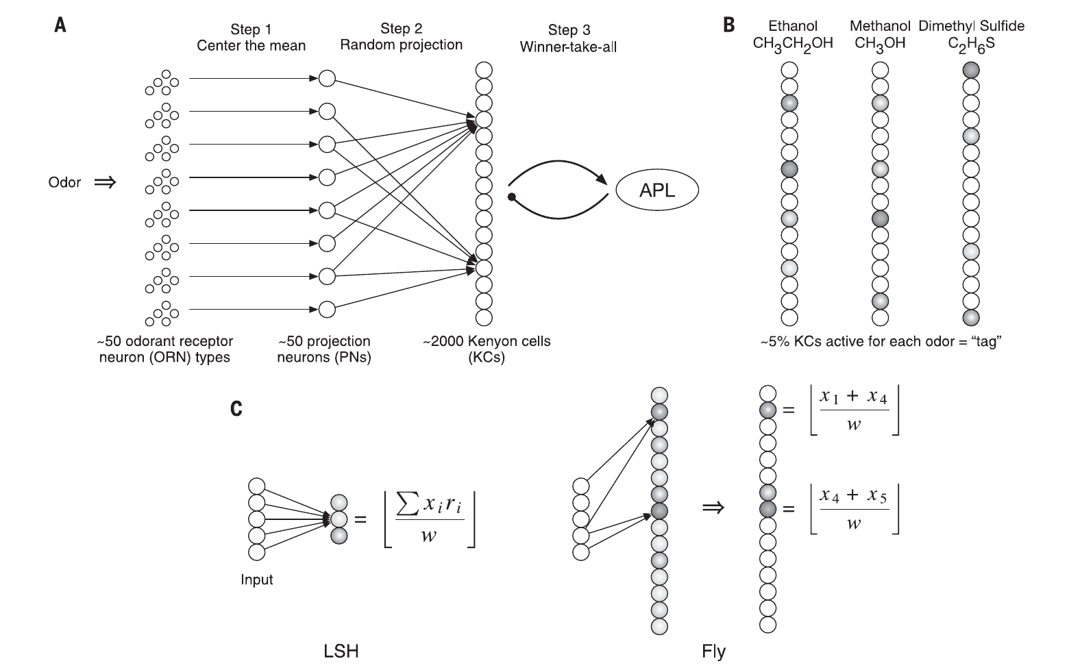
What happens in the fly
In the fly, smell is not represented as a single scalar like "banana" or "danger." Odor molecules activate receptor neurons, those signals are organized into glomeruli in the antennal lobe, and projection neurons carry a compact odor pattern into higher brain areas. The mushroom body then performs the part that matters for this post: it expands that compact pattern into many Kenyon cells, keeps the response sparse, and gives downstream neurons a clean tag to learn from.
Plainly: the fly first makes a compact odor vector, then expands it and keeps only a few active neurons.
The important detail from Caron, Ruta, Abbott, and Axel is that individual Kenyon cells receive apparently random combinations of olfactory glomerular inputs. The important detail from Lin and colleagues is that feedback inhibition helps keep Kenyon-cell odor responses sparse and decorrelated.
Detect and compress
Odor receptors feed the antennal lobe. Glomeruli turn a chemical mixture into a compact population pattern.
Expand randomly
Projection-neuron activity fans into the mushroom body. Kenyon cells sample different, apparently random mixtures of glomerular input.
Sparsify hard
High thresholds and APL feedback suppress most Kenyon cells, so each odor leaves a small active tag rather than a dense response.
Read out associations
Downstream mushroom-body output neurons can attach learned value to the sparse tag. In the toy, this is the final readout matrix.
What I intentionally leave out: spikes, timing, receptor chemistry, lateral-horn pathways, dopamine details, and the real mushroom body's cell-type structure. This post only keeps the expansion-and-sparsification algorithmic skeleton.
Plainly: I am borrowing the circuit shape, not trying to model every biological detail.
The toy circuit
Pixels1
\(28 \times 28\) grayscale image. There are \(784\) input numbers.
Flatten2
The image becomes one vector \(x \in \mathbb{R}^{784}\). Nothing has been learned yet.
Sparse random projection3
The projection matrix is \(W \in \mathbb{R}^{F \times 784}\). It creates many random measurements of the same image before the top-k step keeps only the strongest responses.
Expanded activations4
The projection gives \(a = |Wx| \in \mathbb{R}^{F}\). For \(F=64{,}000\), one digit has 64,000 responses.
Keep top 5%5
The dense response becomes \(t \in \{0,1\}^{F}\), with \(\|t\|_0 = 0.05F\).
Readout6
The readout is \(R \in \mathbb{R}^{F \times 10}\), producing \(z = tR \in \mathbb{R}^{10}\).
The toy replaces odors with pixels. The important shape is the bottleneck: a compact image vector becomes a much larger random response, then a tiny sparse tag. The readout only sees that tag.
Why this can work
Random expansion is useful when the sparse tag preserves overlap: two versions of the same digit should share more active cells than unrelated digits. The readout does not need to understand pixels directly; it only needs to attach class evidence to the cells that keep winning together.
Plainly: similar inputs should activate overlapping sparse features, and the readout can learn from that overlap.
The trick is not that random features know the label. It is that expansion creates many possible coincidences, sparsity keeps the strongest ones, and downstream learning can reuse repeated winners as class evidence.
1. Random measurements preserve more than they destroy
The Johnson-Lindenstrauss story says that a random linear map can preserve pairwise distances for a finite cloud of points with surprisingly few dimensions:
Plainly: random projections can keep useful geometry even when the measurements look arbitrary.
\[(1-\epsilon)\|x-y\|_2^2 \leq \|P(x-y)\|_2^2 \leq (1+\epsilon)\|x-y\|_2^2.\]
That theorem is usually stated for dimensionality reduction. Here the direction is flipped: I am using many random measurements as an overcomplete feature map. The same concentration intuition still matters: one random row is noisy, but many random rows give a stable statistical sketch of the input geometry.
Plainly: one random feature is weak, but thousands of them can form a useful sketch.
2. Similar inputs induce correlated responses
If \(x\) and \(y\) are close or aligned, then a random row \(w_i\) tends to give related responses \(w_i^\top x\) and \(w_i^\top y\). For an isotropic random row, the raw dot products are unbiased probes of input similarity:
Plainly: close inputs tend to make the same random tests respond in related ways.
\[\mathbb{E}\left[(w_i^\top x)(w_i^\top y)\right] \propto x^\top y.\]
The absolute value in this toy ignores sign and keeps response magnitude:
\[a_i(x) = |w_i^\top x|.\]
So the random projection is not inventing labels. It is producing many weak, geometry-sensitive tests.
Plainly: the random layer does not know the answer; it only exposes many small clues.
3. Top-k turns weak tests into a sparse locality code
The top-k step keeps only the cells with unusually large responses:
Plainly: keep the strongest responses and turn everything else off.
\[t_j(x)=1[j \in \operatorname{TopK}(a(x))].\]
Now similarity becomes overlap. Two nearby inputs should share more winners, while unrelated inputs should share fewer. This is close in spirit to locality-sensitive hashing: preserve neighborhood structure, not every pixel-level detail.
Plainly: similar examples should share winners; different examples should share fewer.
4. The readout only has to add evidence
Once the tag is sparse, classification can be a sum over active cells:
Plainly: prediction becomes adding up evidence from the few cells that fired.
\[\operatorname{score}_c(x)=\sum_{j:t_j(x)=1} R_{jc}.\]
The class-mean baseline estimates which cells tend to fire for each digit. The delta readout does the same kind of evidence accumulation, but adjusts weights using output error, so it can amplify useful winners and suppress misleading ones.
Plainly: the readout learns which active cells usually help or hurt each digit.
The important caveat is that this only helps if task structure is already visible in the geometry of the input. MNIST has enough geometry that random sparse expansion can expose useful coincidences. A task requiring invariance, sequence memory, or compositional reasoning would need more than this frozen random map.
Plainly: this works best when the raw input already has structure that random features can uncover.
The minimal code
The core of the experiment is just sparse random projection plus a top-k tag. The feature extractor is fixed; only the final readout learns.
Plainly: the random feature layer stays frozen, and only the last layer changes.
acts = abs(X @ W.T)                      # random expanded responses
winners = argpartition(-acts, k - 1)     # top-k Kenyon-cell-like tag

logits = tag @ W_readout
probs = softmax(logits)
err = one_hot(label) - probs
W_readout += lr * tag.T @ err / batch # local readout updateDependencies: NumPy and SciPy for the MNIST run; scikit-learn only if you use the optional --digits smoke test.
What I measured
I swept the number of expanded features F. Each expanded feature samples 12 random pixels, and the code keeps the top 5% active cells. I compared two deliberately simple readouts:
Plainly: I changed the size of the random feature bank and compared two simple ways to read the sparse tag.
- Class-mean baseline: build one prototype tag per digit by counting which cells usually fire for that digit. At test time, score a new tag by summing the prototype values under its active cells and pick the largest score.
- Delta readout: a single local error-Hebbian layer trained from tag activity and output error.
The local readout is much stronger, but the important part is the shape: expansion helps even though the feature map is random and frozen. The class-mean readout saturates early; the learned local readout keeps benefiting at larger capacity.
Plainly: the learnable readout uses the sparse tag better, especially as the random feature bank grows.
Expansion helps the learned local readout more than the class-mean prototype readout. The absolute numbers are not the claim; the useful observation is that a very simple, forward-only feature map creates a tag that a local readout can exploit.
| Expanded features | Active tag size | Expansion | Class-mean baseline | Delta readout |
|---|---|---|---|---|
| 400 | 20 | 0.5x | 59.64% | 76.88% |
| 800 | 40 | 1.0x | 60.87% | 80.00% |
| 2,000 | 100 | 2.6x | 62.76% | 82.52% |
| 4,000 | 200 | 5.1x | 63.24% | 82.75% |
| 8,000 | 400 | 10.2x | 64.21% | 85.11% |
| 16,000 | 800 | 20.4x | 63.99% | 83.48% |
| 32,000 | 1,600 | 40.8x | 64.04% | 87.16% |
| 64,000 | 3,200 | 81.6x | 63.83% | 87.50% |
Fixed \(F=64{,}000\): shrinking the active tag
I also held the random expansion fixed at \(F=64{,}000\) and made the winner-take-all tag smaller. This asks a different question: once the random feature bank is very large, how many active cells does the readout actually need?
Plainly: after making a huge random feature bank, I tested how sparse the active tag can get before accuracy breaks.
With \(F=64{,}000\), the class-mean prototype readout is almost insensitive to \(k\) until the tag gets extremely small. The learned local readout has a broad sweet spot: dense tags are not automatically better, while even \(k=25\), only 0.039% of the feature bank, still reaches 80.40%.
| Active tag size | Sparsity | Class-mean baseline | Delta readout |
|---|---|---|---|
| 25,600 | 40.000% | 64.00% | 83.81% |
| 12,800 | 20.000% | 64.01% | 87.46% |
| 6,400 | 10.000% | 63.85% | 85.64% |
| 3,200 | 5.000% | 63.83% | 87.47% |
| 1,600 | 2.500% | 64.08% | 86.14% |
| 800 | 1.250% | 64.32% | 85.36% |
| 400 | 0.625% | 64.32% | 85.16% |
| 200 | 0.313% | 64.39% | 84.80% |
| 100 | 0.156% | 64.32% | 84.04% |
| 50 | 0.078% | 63.92% | 82.60% |
| 25 | 0.039% | 63.22% | 80.40% |
Why this is interesting
The usual deep learning move is to learn the feature extractor end-to-end. This toy goes the other direction: spend a lot of cheap random features, sparsify hard, and ask whether the resulting tag is already useful.
Plainly: instead of learning features, this asks how far fixed random features can get.
That is why I like the fly analogy. Expansion and sparsity are not just implementation details; they are a bet about representation. A random dense projection smears everything. A sparse expanded tag gives downstream learning a high-dimensional set of coincidences to attach meaning to.
Plainly: sparse expansion gives the readout many reusable hooks instead of one blurred representation.
The next question is not "can this beat a CNN on MNIST?" It should not. The next question is which parts of the trick survive when the task needs invariance, temporal order, or continual learning.
Plainly: MNIST is just the sandbox; the real question is whether this trick helps on harder learning problems.
What I am not saying
- This is not a faithful fly model. It is a small artificial circuit inspired by one computational motif.
- This is not state-of-the-art MNIST. A normal CNN will crush it.
- This is not the latest private research direction. It is the safe public scaffold: mechanism, toy code, and measured behavior.
References
- Dasgupta, Stevens, and Navlakha. A neural algorithm for a fundamental computing problem. Science, 2017.
- Caron, Ruta, Abbott, and Axel. Random convergence of olfactory inputs in the Drosophila mushroom body. Nature, 2013.
- Lin, Bygrave, de Calignon, Lee, and Miesenbock. Sparse, decorrelated odor coding in the mushroom body enhances learned odor discrimination. Nature Neuroscience, 2014.
- Johnson and Lindenstrauss. Extensions of Lipschitz mappings into a Hilbert space. Contemporary Mathematics, 1984.
- Dasgupta and Gupta. An elementary proof of a theorem of Johnson and Lindenstrauss. Random Structures & Algorithms, 2003.
- Achlioptas. Database-friendly random projections: Johnson-Lindenstrauss with binary coins. Journal of Computer and System Sciences, 2003.
- LeCun, Cortes, and Burges. The MNIST database of handwritten digits.
- Indyk and Motwani. Approximate nearest neighbors: towards removing the curse of dimensionality. STOC, 1998.
- Rahimi and Recht. Random Features for Large-Scale Kernel Machines. NeurIPS, 2007.